

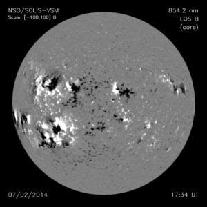
Complex delta sunspot groups such as the one shown above, were observed by me over the Solar Maximum Year (1980) to ascertain whether predictive relationships might be obtained from sunspot morphology.
We now get into the nitty gritty of scientific research and methods to show some of the ways that the nice, neat picture one imagines, e.g. by reading a scientific paper, may actually have been preceded by lots of false leads and wrong conclusions. Or at the very least selection effects that could cast some doubt on conclusions. Take my work in determining the extent to which geo-effective flares could be predicted from sunspot structure. The crux of that work was mainly summarized in a paper appearing in The Journal Of the Royal Astronomical Society of Canada, e.g.
http://adsabs.harvard.edu/full/1983JRASC..77..203S
This was followed by the major paper disclosing the actual relationships between assorted sunspot morphological parameters and flare frequencies, e.g.
http://adsabs.harvard.edu/full/1983SoPh...88..137A
But arriving at the publication was by no means easy or straightforward. First, I had to define exactly the object(s) of inquiry I was seeking: in this case a specific sunspot morphology, i.e. manifested in sunspot groups, that produced solar flares yielding sudden ionospheric disturbances. In addition, I had to identify the SID flares by ensuring every spot group indexed could feasibly be tied (by proximity of heliographic location) to the site of a specific flare with a minimal soft x-ray flux (at SID threshold). This necessitated months of observations of sunspots using the telescope shown above, as well as x-ray, radio and other observations for flares assembled month by month in Solar Geophysical Data.
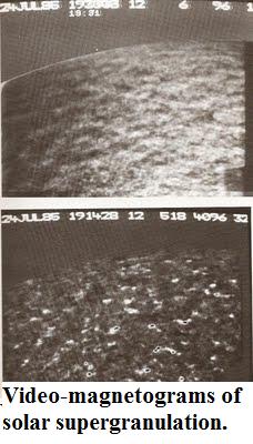
One of the first realizations is that I would have to work with a limited sample set. It was absurd to attempt to look at every sunspot group and associated flare occurring over an entire 11 year cycle. So I limited the sample set to the Solar Maximum Year, which was reasonable and practical.. Other selection effects that entered included: use of Mt. Wilson magnetic classes for identifying magnetic morphology, which are coarse categorizations only; this use in turn introduces a further selection effect with respect to time, i.e. if there is some (SID) flare incidence that occurs in less than a day it would not have been exposed given the Mt. Wilson classes are identified daily only. Also the use of vector magnetograms, such as:
are normally made between 18h00m and 19h00m each day so flares occurring outside this interval (say for rapidly evolving sunspot groups) could lead to a 'mismatched' flare-sunspot magnetic class association. All of these factors were described in the several papers published to do with SID flares.
Other difficulties also emerged and were noted in the papers, including the uncertainties in making an SID flare identification based on its heliographic coordinates relative to the closest sunspot group. In other words, the greater the distance between heliographic coordinates the less secure the identity for the SID generating flare.
Lastly, given that optical images (H-alpha) were used to identify the nearest flares to suspect spot groups, the assumption was made that H-alpha flares could only be in the SID flare category if their emitted soft x-ray flux exceeded 2 x 10 -3 erg cm -2 s -1 (cf. Swider, W. 1979). This assumption necessitated close inspection of the soft x-ray records from the SMS-GOES satellite to ascertain the times for peak emission which later had to be tied to times of optical (H-alpha) flare occurrence. A typical soft x-ray flux record with the SID flares identified by SID and optical importance is shown below:

All this is intended to show that a lot of 'messiness' is involved in scientific research, even to publish a fairly straightforward paper on the associations between sunspots and flares.
Some outside critics might contend the research suffers from another selection effect: excluding all 'no flare' days, instances from consideration. But in 4 subsequent papers, including one published in the monumental 'Solar Terrestrial Predictions Proceedings- Meudon' e.g.

that base was covered. My paper :‘Limitations of Empirical-Statistical Methods of Solar Flare Prognostication’ appearing on pp. 276-284 of the Proceedings showed the limits of prognostication for given (magnetic, optical, radio) observational thresholds. This in turn disclosed the basis for a Poisson-based "delay time" and magnetic energy buildup preceding geo-effective solar flares, paving the way for a flare trigger. This was first postulated by me (Thesis, Proceedings of the Second Caribbean Physics Conference, Ed. L.L. Moseley, pp. 1-11.) to account for release of magnetic free energy using:
¶ / ¶ t {òv B2/2m dV} = 1/m òv div[(v X B) X B] dV
- òv {han | Jms |2 }dV
This paved the way for more accurate forecasts of solar flares, including the geoeffective variety, once optical resolutions for coronal loops attain at least 0.1 arcsec.
We can now examine further examples to show how journal referees can even miss elements that are dissonant or that don't fully support the case being made by the researcher.
1) Jason Lisle's discovery of a "persistent N-S alignment" for solar supergranules:
Sunspots are formed when strong magnetic fields rise up from the convection zone, a region beneath the photosphere that transfers energy from the interior of the Sun to its surface. At the surface, the magnetic fields concentrate into bundles of flux elements or tubes, which prevent the hot rising plasma from reaching the surface, Supergranules, at a scale of nearly 30,000 km across, are among the largest structures supporting the concentration of flux elements via convective downdrafts. And so the "multiple flux tube" model of Eugene Parker was born (cf. Astrophys. J., 230, 905-13).
Very early in his dissertation (p. 17), Lisle concedes an inability to properly resolve granules via his Michelson Doppler Imager (MDI) velocity data, though he does make an appeal to local correlation tracking (LCT) as a kind of savior since it allows motions to be deduced from the images even when individual moving elements aren't well resolved. (I.e. the granules are the individual elements or units of supergranules). The question that arises, of course, is whether this product of such LCT manipulation is real, or to put it another way, an objective physical feature that is not associated with instrumental effects, distortions or errors.
Exacerbating this suspicion is Lisle's own admission (ibid.) that LCT "suffers from a number of artifacts". Indeed. Any central heliographic artifact which sports velocity motions of magnitude 200 m/s - and hence overpowers (by a factor TEN) that signal which one is seeking, is bound to cause havoc and efforts at resolving the signal are likely to be dubious at best...if the right instruments or reduction methods aren't employed.
At least to his credit he admits (p. 21, Thesis) the enormous mismatch between the magnitude of his sought signal and his unwanted artifact noise. He also concedes the artifact is a selection effect and a product of his very LCT algorithm. (The algorithm preferentially selects the central blue-shifted cores of any granules moving toward the heliographic center, and hence exaggerates the associated velocities.)
He claims to be able to "reproduce" the disk-centered false flows and also (presumably by doing this) "account for" many of their properties. But this is disputable, especially given he chooses to replace the velocity component of his LCT flow field with Doppler velocity data. While plausible sounding in theory, in practice it's a different matter, as I learned at the 40th meeting of the Solar Physics Division in Boulder, in 2009. The reason? "Dopplergrams" often betray false motions, by virtue of exhibiting brightness variations in different (spectral) bands which may not always arise from real motions.
Thus, differential brightness changes observed in Dopplergrams may yield motions that are erroneous. This means they can't be used as consistently reliable indices for velocity especially anywhere near the solar photosphere. (At the particular session devoted to Dopplergrams it was pointed out that we need to use maps of subsurface flows in conjunction to obtain accurate readings).
My point here is that if he indeed substituted Dopplergrams to get his velocity component, then he in effect inadvertently added another systematic error on top of his selection errors associated with the large scale flow artifact.
More worrisome are the admissions in the paper he co-authored with Toomre and Rast (Astrophysical Journal paper (Vol. 608, p. 1170), 'Persistent North-South Alignment of the Supergranulation'):
Supergranular locations have a tendency to align along columns parallel to the solar rotation axis.... this alignment is more apparent in some data cubes than others… The alignment is not clearly seen in any single divergence image from the time series of this region (Figs. 1a–1b) but can be detected when all 192 images comprising that series are averaged”
Why should these alignments be more evident in some data cubes than others? Lisle's "solution" is to devise "merit tiles" or tiny sub-sections of data- roughly of meso-granule size (i.e. midway between granule and super-granule) that encompasses the grid points he's selected. He then renders all these merit tiles uniform and with dimensions 5 pixel x 5 pixel, where each pixel scale is ~ 2 arcsec in full disk mode. He asserts this corresponds to 1.4 Mm at the solar center, and "comparable" to the size of a typical supergranule, or 1.0 Mm. However, there is in fact a 40% difference in scale, and what the Dopplergrams velocity profiles will do is increase it.
His next ploy is to resort to "shifting" these tiles by "sub-pixel" amounts in latitude (y) and longitude (x) directions, whereby any tile shifted by delta(x) and delta (y) is compared to the corresponding tile at the same grid point in the in the subsequent image in time. He then claims to be able to evaluate a "correspondence" between any such two tiles according to a "merit function": m(delta(x), delta(y)).
This again is suspect, because if he's using velocity components from Dopplergrams, with their systematic errors (which he doesn't say were ever accounted for) there's no assurance that subsequent tiles will really show the same grid points, far less at the same time (since a systematic delta(v) will shift them). Thus, his "Gaussian weighting function" W, which he then applies to his merit functions (already clearly macguffins) isn't much use.
Going back to the same Ap.J. paper of Lisle et al, the authors write:
“After 8 days of averaging, the striping is quite strong, while shorter averaging times show the effect less well. In Figure 3a, s[x], s[y] , and their ratio s[x]/s[y] are plotted as a function of averaging time. The plots show the average value obtained from two independent well-striped 15 deg x 15 deg equatorial subregions of the data set”
We're also alerted in the same paper to the asymmetrical rms errors for s[x] and s[y]:
s[x]/s[y] shows a smooth transition from values near one at low averaging times to values exceeding 2.5 for the full time series. This increase reflects the slow decrease in x compared to y due to the underlying longitudinal alignment of the evolving flow. The random contributions of individual supergranules to s[x] or s[y] scale as 1/(Nl)^½, where Nl is the number of supergranular lifetimes spanned over the averaging period.
Of course, being unaware of the influence of the anomalous v-component introduced by Dopplergrams this is a natural conclusion to make, that is, that a preferential persistence is displayed in x as opposed to y. However, if the Dopplergrams have introduced systematic errors in v as I am convinced, it is more plausible that we are seeing the emergence of asymmetric ERRORS in s[x] over s[y]. (Such that s[x] ~ 2.5 s[y]].
The confirmation of this spurious effect for me is when the authors write:
Vertical striping of the average image emerges visually when the averaging time exceeds the supergranular lifetime by an amount sufficient to ensure that the contribution of the individual supergranules falls below that of the long-lived organized pattern.
In other words, to control the signal to obtain the effect they need they have to resort to time averages t(SG) < T(P), where T(P) denotes the lifetime of the organized pattern.
How would they have fared better, and uncovered the likely systematic error in v from the Dopplergrams? They ought to have applied the statistical methods described by James G. Booth and James P. Hobert ('Standard Errors of Prediction in Generalized Linear Mixed Models', appearing in The Journal of the American Statistical Association (Vol. 93, No. 441, March 1998, p. 262) in which it is noted that standard errors of prediction including use of rms errors, and ratios thereof are "clearly inappropriate in parametric models for non-normal responses". This certainly appears to apply to Lisle et al's polarity "model" given the presence of significant "false flows" and "large convergence artifacts" (the latter with 10 times the scale size of the sought signal).
Until this is done, it cannot be said that there exists any "persistent alignment" in the solar supergranulation.
2) The Adoption of a "Dynamo Model" to Describe Solar Flares Based On Auroral Mechanisms.
Here I focus on one particular model - the "Dynamo Flare" model of Kan et al(Solar Physics, Vol. 84, p.153, 1983) and show how it misses the boat. While Kan et al’s Dynamo model commendably incorporates both energy generation and dissipation, it exhibits a number of defects which translate into a hidden “cost” for using unobserved structures, processes. In general, their model overtaxes the similarity between substorms and solar flares, while ignoring key facts concerning the magnetic aspect of flares – such as the well-established relationship between magnetic complexity and important flares (e.g. Tanaka and Nakagawa.: Solar Physics, Vol. 33, p. 187, 1973)
Some major divergences:
i) "Neutral wind":
In the Dynamo model of Kan et al (1983), the “neutral wind” acts perpendicularly to the field –aligned ( J ‖ ) and cross-field (J ⊥ ) current, see e.g. their model structure below:
The wind is described in their paper as a “shear flow” (p. 154) . The problem is that there is no evidence of such “neutral gas” in the region of the solar chromosphere or photosphere, nor of any consistent “flow” of the order of 1 km/s. Thus, it is an entirely fabricated construct bearing no similarity to real solar conditions. (Of course, adopting the positivist stance the authors can argue like Hawking does in his quantum coherence theory, that there is no correspondence to physical reality anyway, and it is only used to make predictions.)
More accurately, in the regions wherein real magnetic loops reside, the physical features of sunspots and their concentrated flux dominate. Thus, instead of some vague “neutral wind’ one will expect for example, a convective downdraft which helps to contain the individual flux tubes of a sunspot in one place (e.g. Parker, Astrophysical. J., 230, p. 905, No. 3, 1979.) The problem is that the downdraft velocity is not well-established and can vary from 0.3 to 1.5 km/s.(Parker, op. cit.)
In the proper space physics (magnetopheric) context, the “neutral wind” arises from a force associated with the neutral air of the Earth’s atmosphere (e.g. Hargreaves, The Solar-Terrestrial Environment, Cambridge Univ. Press, 1992, p. 24). This force can be expressed (ibid.):
F = mU f
where f is the collision frequency. It is also noted that this wind blows perpendicular to the geomagnetic field (ibid.)
If one solves for f above, and uses the magnitude of magnetic force (F = qvB) where B is the magnetic induction, and v the velocity one arrives at two horizontal flows for electrons and ions moving in opposite directions. mU f = qvB = (-e) vB = (e) vB
Thus,
v1 = mU f / (-e) B and v2 = mU f / (e) B
These ions and electrons thus move in opposite directions, at right angles to the neutral wind direction. Such “neutral wind” velocities are depicted in Kan et al’s Fig. 1 (into and out of the paper on the right side of their arch configuration) as ±V_n. In the magnetospheric system the current is always extremely small since the frequency is large. (Hargreaves, ibid). The region where the wind is most effective in producing a current in this way is known as “the dynamo region”.
Again, there is no similar quasi-neutrality in the solar case, since the ions and electrons move as one governed by the magnetic field in the frozen-in condition. This shows that the whole neutral wind concept has no validity in the solar magnetic environment.
ii) Plasma motions – Lorentz force (J ⊥ X B)
In Kan et al’s (1983) dynamo flare model, predicated on space physics concepts, it is required that the dynamo action send currents to specific regions to provide a Lorentz force: (J ⊥ X B). This implies a current system which is non-force free in contradiction to numerous existing observations, and the fact that at the level of the photosphere –chromosphere, the plasma beta:
b
= r v2 m/ B2
is much less than 1.
For example, contrary to their claim that the currents in the chromosphere are not parallel to the magnetic field, we have actual vector magnetographs which show otherwise. For example, gyro-resonance emission depends on the absolute value of the magnetic field in the region above sunspots, and contour maps of such regions at discrete radio wavelengths disclose the controlling influence of magnetic fields. Penumbral filaments of sunspots themselves lie in vertical planes defined by the horizontal component of the magnetic field .
Again, both coronal and chromospheric gas pressures are insignificant relative to magnetic pressures, so fields in these regions must be at least very nearly force-free.
In the case of filaments or prominences in the low corona or chromosphere, the plasma as we saw before, would again have a very high magnetic Reynolds number, Re(m). The conductivity of the plasma would therefore be ‘infinite’ so that even a minuscule induced voltage arising from, E = -v X B (e.g. due to very small relative motion v) would produce an infinite current j = s E. The only way one avoids this unrealistic situation is to require the plasma motion in the filament to follow magnetic field lines rather than cut across them.
Clearly, the error being made in this case and others is the overextension of space physics structures and concepts (e.g. as applicable to the aurora) to the solar physics – and specifically the solar flare, context. To be more precise, one can visualize (in the case of the aurora) bundles of open field lines that map to the region inside the auroral oval. Many of these field lines can be traced back to the solar wind. The configuration is such that one is tempted to conceive of a mechanism that links certain mechanical or dynamic features to the production of cross currents, including Birkeland currents.
In detailed auroral models it can be shown that the "dynamo currents" in such a process flow earthward on the morning side of the magnetic pole and spaceward on the evening side. The circuit can be visualized completed by connecting the two flows across the polar ionosphere, from the morning side, to the evening side. This is exactly what Kan et al have done in arriving at their “dynamo solar flare” model. That is, taken a mechanism that might be justified in the case of the aurora – and transferred it to the solar flare situation.
The problem inheres in the fact that circuits on the Sun – given unidirectional current flows – need not be driven by any “dynamo action” – or be part of any dynamo. Further, one doesn’t require a dynamo to have a conservative energy system to account for solar flares. It is possible to use the conservation of magnetic helicity in a more general context to explain energy balance – especially for large, two-ribbon flares.
In addition, it should be obvious even to a non-scientist that each example embodies relative truth, in this case scientific truth. This goes back to my earlier post on the degree to which one can approach "absolute" truth. Well, at least in science, not that closely because all scientific methods ultimately depend on empirical results and these are subject to change. They are also employed by fallible humans - not 'gods' - subject to errors, inconsistencies and false assumptions.
As anyone who does scientific research knows, it
is quite impossible to "prove" a particular solution to a scientific
problem to be "true" (that is, true for all times and
conditions). Solutions of scientific
problems are instead assessed for adequacy,
that is, in respect to the extent to which the researcher's stated aims have
been carried out. Two categories of criteria are those related
to argument and to the evidence presented. To judge adequacy then, we look for the
strength and consistency of logical/mathematical arguments, and the goodness of
fit of the data in a given context. By
"goodness of fit" I mean that two different datasets on comparison
are either strongly correlated or anti-correlated.
All such determinations of adequacy perform the same function for scientific research that quality control does for industry. Most importantly, no determination of adequacy can be rendered until and unless the research is published in a refereed journal. However, even if research is published, this only meets the first threshold for objective acceptance. One must then be able to check the research over time to ascertain the extent to which it supports further observations or experimental results.
Of course, different theories of science
represent different levels of abstraction:
quantum theory is at a higher level than general relativity, and general
relativity is at a higher level than Newton's theory of gravitation. But-- and here is the key point-- the limits of validity for each theory are
ultimately founded in measurements,
specifically through careful experiments carried out to test predictions.
Alas, many non-specialist authors confuse abstraction with lack of QA testing or supporting evidence. For example, in their recent book 'Bankrupting Physics: How Today's Top Scientists Are Gambling Away Their Credibility', Alexander Unzicker and Sheilla Jones claim today's physicists regularly announce major discoveries with little meaningful evidence to support the claims. I noted some of these sort of problems in regards to the discovery of the Higgs boson, e.g.
http://brane-space.blogspot.com/2013/10/god-particle-theorists-get-nobel-prize.html
The two authors (one a German HS teacher and science writer, the other a Canadian science journalist) also claim the scientific method has been "swept aside" - but in fact no such action has been done. It is merely that the methods employed have been more theoretical and mathematical than observational -experimental. (And the experimental results as have been disclosed, as in the case of the Higgs, still leave questions unanswered.)
The point also needs to be emphasized that the greatest theories of the 20th and 21st century remain theoretical in basis and also the most accurate. As pointed out by Roger Penrose ('The Nature of Space and Time', p. 61), quantum field theory (QFT) is accurate to "about one part in 10-11" and general relativity has been "tested to be correct to one part in 10 -14 ". In other words, if the scientific method had been swept aside for such abstract theories those levels of accuracy would never have been attained. The argument isn't about whether the scientific method pertains to a branch of physics, say, but rather the exact nature of the testing of reality done according to the method used.
It is this testing of reality which provides a
coherent basis for scientific claims, and which bestows on science a legitimacy
founded in reality rather than wish fulfillment fantasies. This is the most important point that readers need to take away. All the examples illustrated for research test reality in some way, but the question that remains is to what degree did each succeed. My point, and I believe that of Wolpert and Baggini, is there is no uniform standard for meeting that success.
This is not to imply that some or all of a given published scientific research paper is necessarily "wrong" but rather that one must take care in reading journal papers - of whatever discipline. This is to ensure confidence that what the author(s) are claiming, i.e. a novel discovery, is valid. Also, if a finding is perhaps incomplete or leaves questions unanswered then these open venues for further investigation. This is the nature of science, approach to truth by successive approximations, not successive "proofs".
Above all, in any research, there are always going to be many assumptions made and certainly if the authors don't come out and state them, the reader must be able to ascertain them - at least to a degree. Indeed, a savvy reader may be able to spot unsupported assumptions (even errors of fact or statistics) the journal peer review missed.
Again, bear in mind science is a limited enterprise carried out by fallible beings subject to their own biases and even prone to errors, or errors that may be overlooked on account of a confirmation bias. Never mind, science is still the best means we have to test reality!
No comments:
Post a Comment